Background
Automatic differentiation is a method for automatically evaluating the derivative of a function for a given input. It is similar to symbolic differentiation and numerical differentiation. Unlike symbolic differentiation which yields a function given an input function of which we would like to take the derivative, automatic differentiation simply yields the derivative evaluated at the given input (rather than the symbolic representation of the actual derivative).
Numerical differentiation, or finite difference approximation, is a rather simple technique for approximating the derivative at a given point by also computing the output for inputs close to the given value and computing the slope. That is, if we want to compute the derivative at a given point, say x, we evaluate the function for some x+e where e is some small value and then compute the slope using x, x+e, f(x) and f(x+e).
In this post, we will be exploring automatic differentiation in NetsBlox, a visual blocks-based programming language.
The Basics
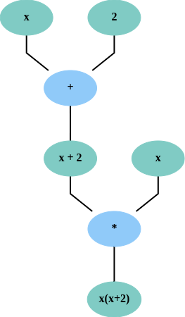
Before we start, we should cover the basic idea of automatic differentiation. Essentially we will be defining functions for the basic mathematical operations which not only compute the consequence of applying the given mathematical operation but they will also construct a computational graph. The computational graph is a graph representation of all the mathematical operations performed on a given value. A simple example of a computation graph computing x(x+2) is shown below. In the figure, operations are represented by blue nodes and operands by green nodes:
We can now compute the gradient by recursive application of the chain rule on the computation graph. There are two different approaches to automatic differentiation: forward mode and backward mode differentiation. These modes correspond to the direction in which the chain rule is applied in the computational graph. In forward mode, the chain rule is applied recursively from the inner-most operation (performed directly on the independent variable to the final output - usually this means from x to y). As the name suggests, in backward mode this is performed in the opposite direction (from the dependent variable to the independent). For a more thorough explanation of automatic differentiation, check out the wikipedia page.
Implementing Automatic Differentiation in NetsBlox
In order to implement automatic differentiation in NetsBlox, we will need to create a custom representation of (differentiable) numbers that builds up a computation graph when mathematical operations are performed on them. That is, rather than simply returning the output of the given operation, we will need to include the output, derivative of the given operation, and store references from the inputs to the outputs of the operation. As complex data structures are represented as heterogenous lists in NetsBlox, we will be replacing simple numbers with a list representation of the value (with the beforementioned side information).
To promote ease of use of these data structures, we will provide additional blocks for interacting with them:
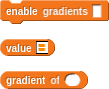
As we will be representing numbers with lists, the above blocks will be used to hide some of this complexity. That is, the enable gradients block will be used to convert a number to a data structure recording the computational graph and gradient. value will be used to get the actual numeric value of one of these data structures and gradient of will be used to get the gradient of a variable, as the name suggests.
As we are representing differentiable numbers as lists, we will also need to provide custom implementations of our mathematical operations. These operations will need to not only compute the result of the operation but also record edges in the computational graph and gradients for each input (with respect to only the given operation). To improve the legibility of the individual mathematical operations (and reduce code duplication), I will be using the following block as a helper block to create differentiable values. This block creates the differentiable value (represented as a heterogeneous list) from the beforementioned three values: output of the value of the operation, gradients with respect to the inputs, and the inputs (to create the reference from the inputs to the outputs). Specifically, this helper function outputs a new differentiable number (set to the output of the mathematical operation) and then records the gradient and a reference to this output for each input.

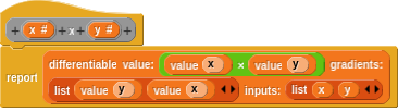
Using this helper method, we can now easily create mathematical operations for our differentiable values. One such example is provided below. In this example, we are defining multiplication on our differentiable values. The output value is clearly the product of the numeric values of the inputs. The gradients are simply the numeric values of each of the inputs (ie, the partial derivatives with respect to each input) and then we also pass the inputs themselves so that they can include a reference to the output.
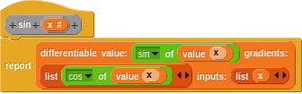
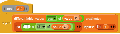
Analogous custom blocks can be created for operations like sine and cosine:
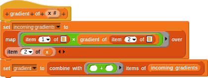
Once we have our representation for differentiable values and mathematical operations defined on these values, we can actually implement the gradient computation. As mentioned before, a differentiable number is represented as a list where the first item is the value of the list and the second is a list of gradients and subsequent nodes in the computation graph. That is, the second item of a differentiable value (represented as a list) is a list of gradients and subsequent nodes in the computation graph. This makes a naive implementation of the gradient computation relatively straight-forward:
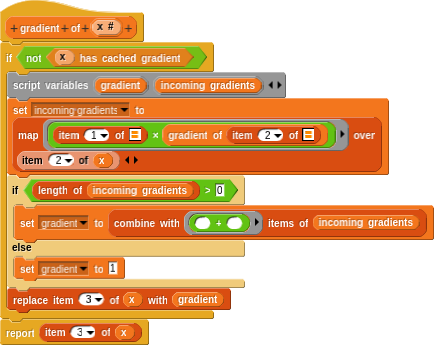
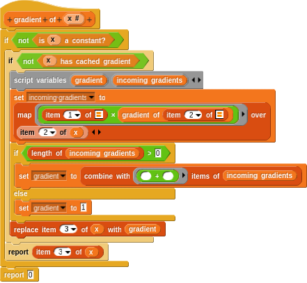
Of course, if a variable has no operations performed on it, the gradient is simply 1. Furthermore, we can cache the computed gradient for a variable in the third item of the list. This results in the following updates to the gradient computation:
Finally, we can ensure that this function trivially returns 0 when computing the gradient of a constant:
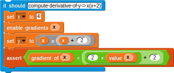
Now, we can give it a try by chaining a couple simple operations and verifying that the gradient is computed correctly! Although there is some code below demonstrating a simple test case, it is a bit more interesting to view an interactive example!